LLaVA-NeXT: What Else Influences Visual Instruction Tuning Beyond Data?
Table of Contents
Visual instruction tuning plays a crucial role in the advancement of large multimodal models (LMM), which aim to follow human intentions to complete diverse computer vision tasks in the wild. In this line of research, studies have consistently demonstrated the effectiveness of a data-centric approach in achieving success, highlighting the importance of high-quality instruction data, as demonstrated by the progression of the LLaVA family, including LLaVA-1.0, LLaVA-1.5, and LLaVA-NeXT, the latest iteration released in Jan. & May. In particular, the largest LLaVA-NeXT-110B model shows near GPT4-V performance on selected benchmarks, achieved through a cost-effective training recipe. Nonetheless, fewer studies have been reported to elucidating the impact of additional factors within the recipe. It raises the question: what else influences visual instruction tuning beyond the instruct data itself?
In this blog post, we present a comprehensive ablation study aimed at addressing these overlooked aspects and augmenting prior insights:
- Architectures: The LLaVA architecture consists of a pre-trained LLM and a pre-trained vision encoder. The model size scaling of LLM is more effective than image encoder in yielding improved performance. The success of the latter is more related to its visual input configuration (resolution, #token) than its model size.
- Visual Representations: The representation of visual signals relates to both the resolution in the raw pixel space and the number of tokens in the feature space. The scaling of both factors leads to improved performance, especially on tasks that require visual details. To strike a balance of performance and cost, we observe that the scaling of resolution is more effective than the scaling of token numbers, and recommend an AnyRes strategy with pooling.
- Training Strategies: In complementary to prior LLaVA series that focus on visual instruction tuning stage only, we explore the impact of training strategies in LLaVA's earlier model life cycle, by varying training data amount, quality, and trainable modules. Our findings suggest the significance of incorporating a stage focused on learning from high-quality knowledge, as opposed to web-scale low-quality data. Specifically, this involves training the entire model using synthetic high-quality data, re-captioned by LLaVA-NeXT-34B.
[Notes on Image Detailed Caption and Video Detailed Caption Tasks.]
Since there is no existing benchmark for evaluating a model's image detailed captioning ability, and we consider this capability crucial for our model's development. For example, it could determine if the model can serve as a proficient detailed captioner for data re-captioning tasks. To address this need, we have constructed two tasks:
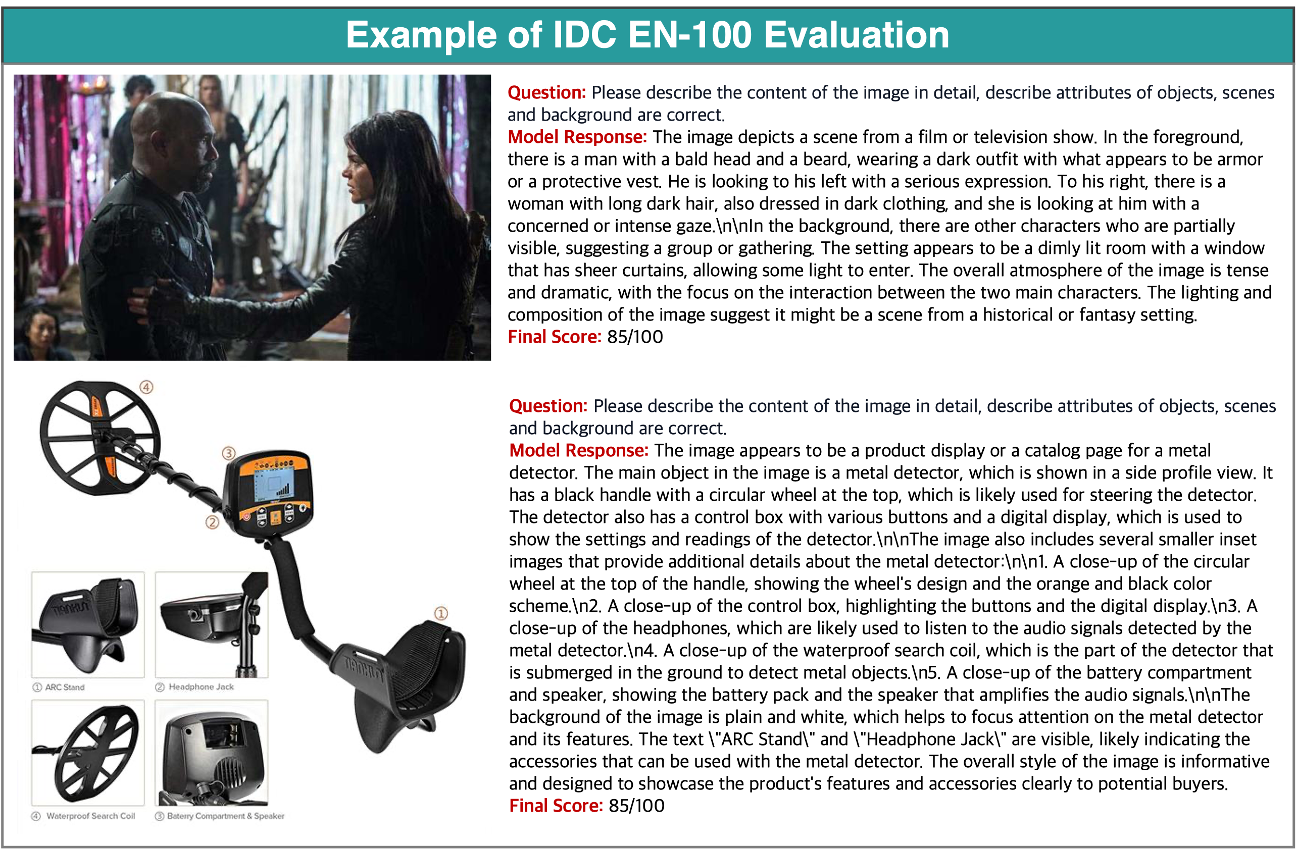
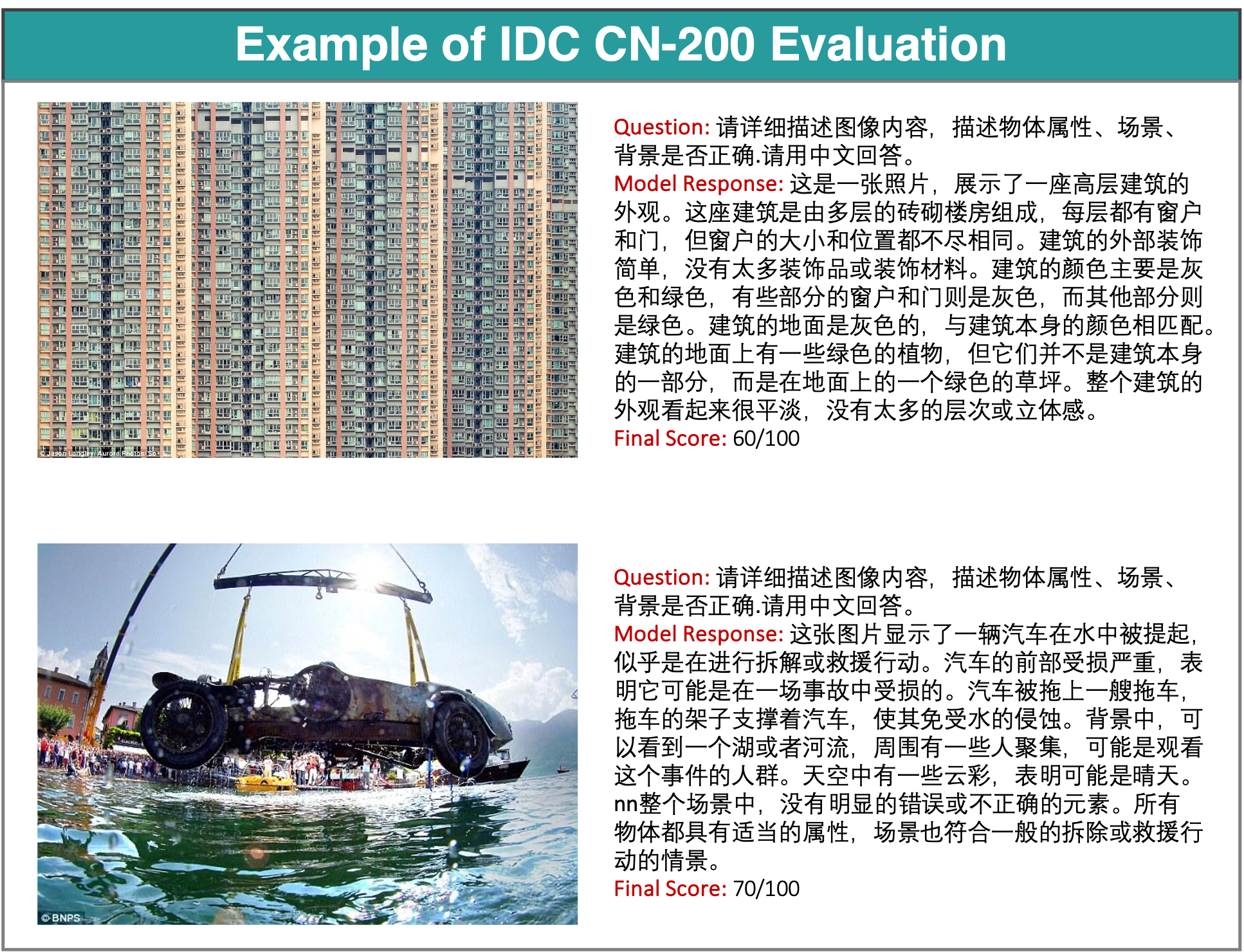
- Image Detailed Caption Task: We collected 100 instances for English detailed captions and 200 instances for Chinese detailed captions, requiring the model to generate highly detailed descriptions. GPT-4V is used to assist with scoring.
- Video Detailed Caption Task: To assess the model's temporal detailed captioning ability, we referred to the VideoChatGPT evaluation and selected 499 questions. The model generates detailed descriptions, which are then scored using GPT-3.5-Turbo and ground-truth comparisons.
The datasets and evaluation process is detailed in the Dataset Card section.
Opensource Release
Re-captioned Data with LLaVA-NeXT-34B is available on Hugging Face Datasets.
Section 1 - Insights on Architectures
The LLaVA architecture is composed of two pre-trained modules: an LLM and a vision encoder. Both modules encode rich knowledge, thanks to the large volume of training data they have been exposed to and the computational resources utilized throughout their model life cycles, respectively. Consequently, the scaling behavior (in terms of model size and data size) of LMM may differ from that of LLMs trained from scratch[1,2,3], when only the LMM training stage is considered, without taking into account the LLM and vision encoder cost. For LMM, we have shown stronger LLM leads to better multimodal performance in the wild in our previous blog, demonstrating the significant improvements of LLaVA-NeXT-110B. In this blog, we systematically study model size scaling behavior.
[Fold / Unfold to See the Details of Baseline Experiment Settings with CLIP-L-336 + Vicuna-1.5 7B]
| Configurations | ||
|---|---|---|
| Architecture |
Image Encoder: OpenAI CLIP-Large (336x336) Connector: 2-Layer Relu MLP LLM: Vicuna-1.5 7B |
|
| # Total parameters | 7.06B | |
| Visual Representations | Dynamic: 336 x {2×2,1×{2,3},{2,3}×1} | |
| Stage-1 | Training Data | 558K |
| Trainable Module | Connector | |
| Stage-2 | Training Data | 790K |
| Trainable Module | Full model | |
| Training Data (# samples) | 1348K = 558K+790K | |
| Training Schedule | Learning rate | LLM: 2e-5 / Vision: 2e-6 |
| Batch Size | 128 | |
Section 1.1 - Language Models
We report several interesting observations and useful tips for LMM practitioners:
- Larger LMs. Multimodal performance has a strong correlation with language model performance, as scaling LLMs directly demonstrate free gains in multimodal performance across all benchmarks. This suggests that development of stronger language model capabilities accumulates richer language knowledge, easily improves the model's multimodal capabilities probably due to cross-modality generalization. It can potentially reduce the need for extensive additional training specific to multimodal tasks, whose high-quality data might be more difficult data to obtain.
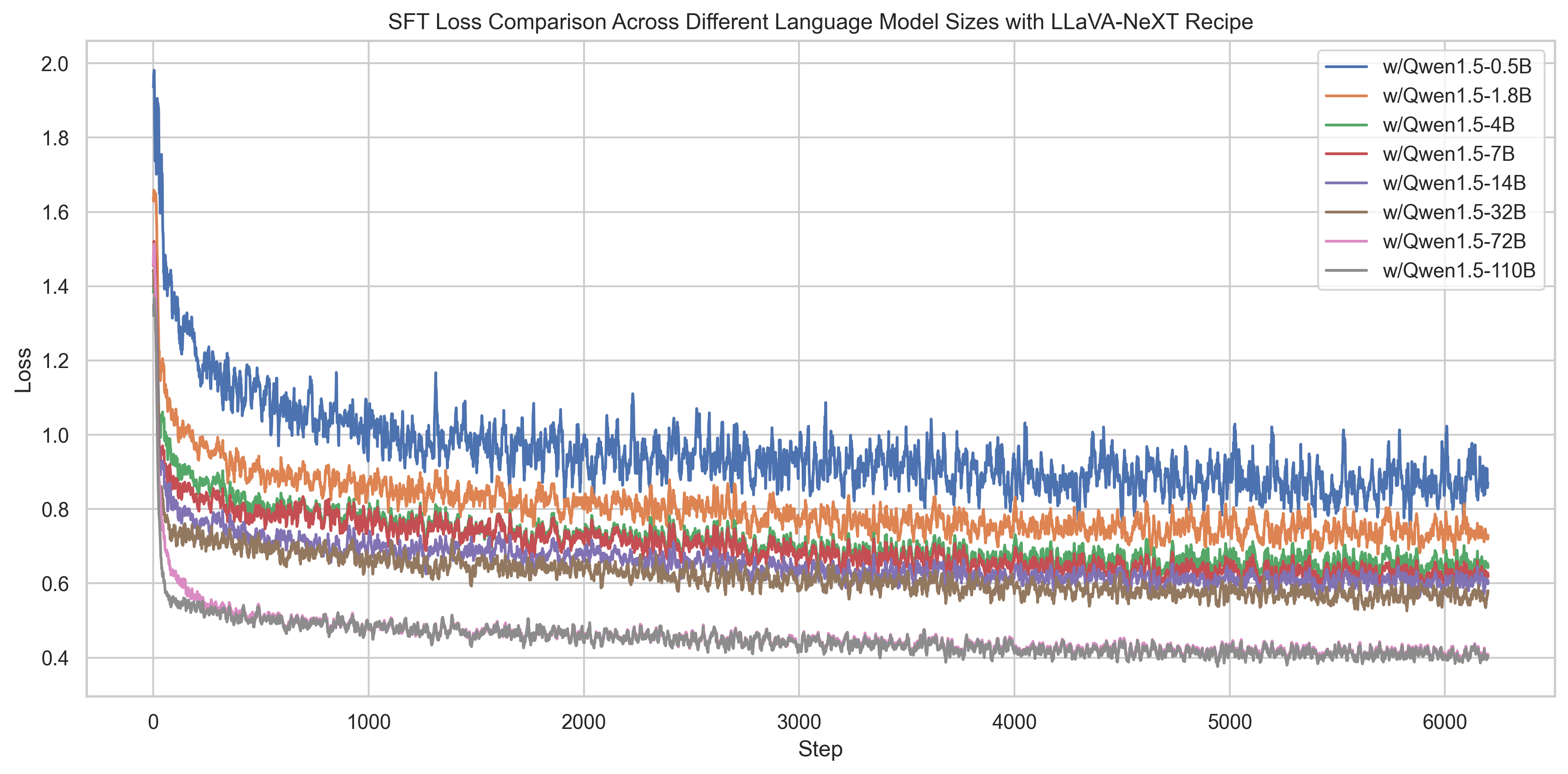
- Lower training loss. Larger LMs converge faster and reach to lower loss values more easily. This is likely because larger models have a greater capacity to learn more complex patterns and store richer language knowledge, leading to faster convergence and better generalization, respectively. Typically, we observe that training curves can be used to monitor the learning process: lower loss values indicate improved performance across a range of tasks.
- Learning rate adjustments. Larger LMs require a smaller learning rate to avoid issues of unstable training dynamics. We observed that the spikes in training curves often indicate worse performance even when the loss values converge to the same. Lowering the learning rate can alleviate the issue. We experimented with a range of learning rate combinations for LLMs and the vision encoder in the format of (LLM, Vision) , including (2e-5, 2e-6), (2e-5, 1e-6), (1e-5, 2e-6), (1e-5, 1e-6), (5e-6, 1e-6), and (5e-6, 5e-7). We found that the vision encoder's learning rate should always be 10x or 5x smaller than the LM decoder's learning rate to stabilize training. Although we didn't observe significant differences in loss values when tweaking the LLM's learning rate from 2e-5 to 5e-7, the final performance on evaluation benchmarks varied significantly.
| LLM Decoder | Batch Size | Learning Rate | Avg. | AI2D | ChartQA | DocVQA | MathVista |
*MME | MMMU |
LLaVA-W | ScienceQA | **Image-DC | |
|---|---|---|---|---|---|---|---|---|---|---|---|---|---|
| LLM (Qwen-1.5) | Vision | - | test | test | val | testmini | - | dev | - | IMG | EN-100 | ||
| 0.5B | 128 | 2e-5 | 2e-6 | 52.8 | 49.4 | 54.8 | 63.4 | 28.1 | 57.0 | 29.4 | 61.7 | 60.0 | 71.6 |
| 1.8B | 57.6 | 59.5 | 58.2 | 67.6 | 29.3 | 55.8 | 32.8 | 69.7 | 66.0 | 79.7 | |||
| 4B | 63.7 | 68.6 | 65.2 | 73.8 | 34.5 | 63.6 | 36.4 | 76.1 | 70.8 | 83.9 | |||
| 7B | 65.2 | 73.5 | 68.5 | 75.7 | 32.1 | 65.1 | 37.4 | 76.4 | 72.5 | 85.2 | |||
| 14B | 70.7 | 75.8 | 71.5 | 80.8 | 41.2 | 69.9 | 43.3 | 86.6 | 77.5 | 89.5 | |||
| 32B | 1e-5 | 72.7 | 76.3 | 74.0 | 79.8 | 42.6 | 69.8 | 48.9 | 90.8 | 81.5 | 91.0 | ||
| 72B | 74.0 | 77.4 | 77.0 | 84.4 | 46.6 | 77.1 | 46.4 | 89.2 | 83.9 | 94.3 | |||
| 110B | 76.0 | 80.4 | 79.7 | 85.7 | 49.0 | 78.6 | 49.1 | 90.4 | 83.2 | 95.5 | |||
*Throughout our blog's presentation, we convert MME's score to accuracy by summing up the perception and cognition scores and dividing 2800.
**Image Detailed Caption Task is a new benchmark we constructed to evaluate the model's detailed captioning ability towards given images. The task is described in the Datasets Card section.
[Fold / Unfold to See the Impact of Batch Size Across Different LLM Size]
| LLM Decoder | Batch Size | Learning Rate | Avg. | AI2D | ChartQA | DocVQA | MathVista |
*MME | MMMU |
LLaVA-W | ScienceQA | Image-DC | |
|---|---|---|---|---|---|---|---|---|---|---|---|---|---|
| LLM (Qwen-1.5) | Vision | - | test | test | val | testmini | - | dev | - | - | EN-100 | ||
| 0.5B | 64 | 2e-5 | 2e-6 | 54.1 | 49.3 | 55.0 | 63.2 | 28.6 | 65.4 | 29.6 | 63.9 | 59.8 | 72.0 |
| 128 | 54.0 | 49.4 | 54.8 | 63.4 | 28.1 | 67.3 | 29.4 | 61.7 | 60.0 | 71.6 | |||
| 1.8B | 64 | 58.7 | 60.0 | 59.3 | 68.0 | 29.7 | 65.4 | 32.8 | 70.2 | 65.1 | 78.0 | ||
| 128 | 58.7 | 59.5 | 58.2 | 67.6 | 29.3 | 65.8 | 32.8 | 69.7 | 66.0 | 79.7 | |||
| 4B | 64 | 63.7 | 68.7 | 65.7 | 74.3 | 33.0 | 73.2 | 35.0 | 71.5 | 69.8 | 82.2 | ||
| 128 | 64.9 | 68.6 | 65.2 | 73.8 | 34.5 | 75.0 | 36.4 | 76.1 | 70.8 | 83.9 | |||
| 7B | 64 | 66.1 | 72.5 | 68.6 | 77.2 | 33.5 | 75.8 | 37.3 | 74.5 | 69.0 | 86.6 | ||
| 128 | 66.5 | 73.5 | 68.5 | 75.7 | 32.1 | 76.8 | 37.4 | 76.4 | 72.5 | 85.2 | |||
| 14B | 64 | 71.7 | 74.5 | 73.2 | 80.8 | 39.3 | 82.7 | 42.6 | 86.8 | 76.4 | 89.1 | ||
| 128 | 72.1 | 75.8 | 71.5 | 80.8 | 41.2 | 82.4 | 43.3 | 86.6 | 77.5 | 89.5 | |||
[Fold / Unfold to See the Impact of Training Loss Curves Across Different LLM Size]
Section 1.2 - Vision Encoders
We consider using different vision encoders in the following experiments for further research. In the table below, we highlight the differences among various vision encoders. These differences include encoder model size, resolution, # visual tokens, and pretraining data. The LLM training time required when integrating them into the LMM also varies significantly.
We make the following observations:
- For vision encoders in LMM, the visual representation on (resolution, #token) and pre-training data play a more significant role than model size. This is because visual representations allow encoding more visual details, and pretraining data allows the model to encode more visual knowledge. The model size with contrast loss shows less scaling gains.
- As a cost and performance trade-off, SO400M shows the most significant advantages. Its large pretraining data (WEBLI-10B), high pretraining resolution (384 x 384), and the number of visual tokens it can express are likely the reasons for its superior performance when integrated into the LMM.
| Vision Encoder | Model size | Res. | Visual Tokens | Pretrained Data | Time Cost | Avg. | AI2D | ChartQA | DocVQA | MathVista | MME | MMMU | LLaVA-W | ScienceQA | Image-DC | ||
|---|---|---|---|---|---|---|---|---|---|---|---|---|---|---|---|---|---|
| Source | Amount | Seen Samples | - | test | test | val | testmini | - | dev | - | IMG | EN-100 | |||||
| CLIP-L | 0.3B | 224 | 256 * 5 | WIT | 0.4B | 13B | ~12H | 63.4 | 67.0 | 60.3 | 62.2 | 33.5 | 78.8 | 38.2 | 71.7 | 71.9 | 86.7 |
| CLIP-L | 0.3B | 336 | 576 * 5 | WIT | 0.4B | 13B | ~30H | 65.3 | 67.4 | 65.2 | 74.5 | 35.4 | 77.3 | 36.6 | 72.6 | 71.0 | 87.6 |
| EVA-02-E | 4.7B | 224 | 256 * 5 | LAION | 2B | 9B | ~30H | 61.0 | 66.9 | 42.4 | 65.4 | 33.5 | 77.5 | 33.6 | 73.9 | 69.5 | 85.9 |
| EVA-8B | 8B | 224 | 256 * 5 | LAION + COYO | 2B | 9B | ~24H | 63.3 | 67.8 | 56.0 | 66.3 | 32.1 | 77.1 | 35.0 | 75.9 | 71.5 | 88.0 |
| EVA-8B | 8B | 448 | 1024 * 5 | LAION + COYO | 2B | 9B | ~75H | 64.4 | 68.4 | 59.7 | 69.8 | 33.4 | 77.3 | 34.6 | 74.4 | 71.9 | 90.2 |
| SO400M | 0.4B | 384 | 729 * 5 | WebLI | 10B | 40B | ~36H | 66.4 | 69.4 | 62.7 | 72.5 | 35.1 | 76.5 | 34.8 | 85.8 | 72.4 | 88.8 |
Section 2 - Visual Representations
The visual representations relate to both the resolution in the raw pixel space and the number of tokens in the feature space. Scaling either of them improves performance, but also introduces computation overhead. This section aims to investigate the best (resolution, #token) configuration for a balance of performance and cost.
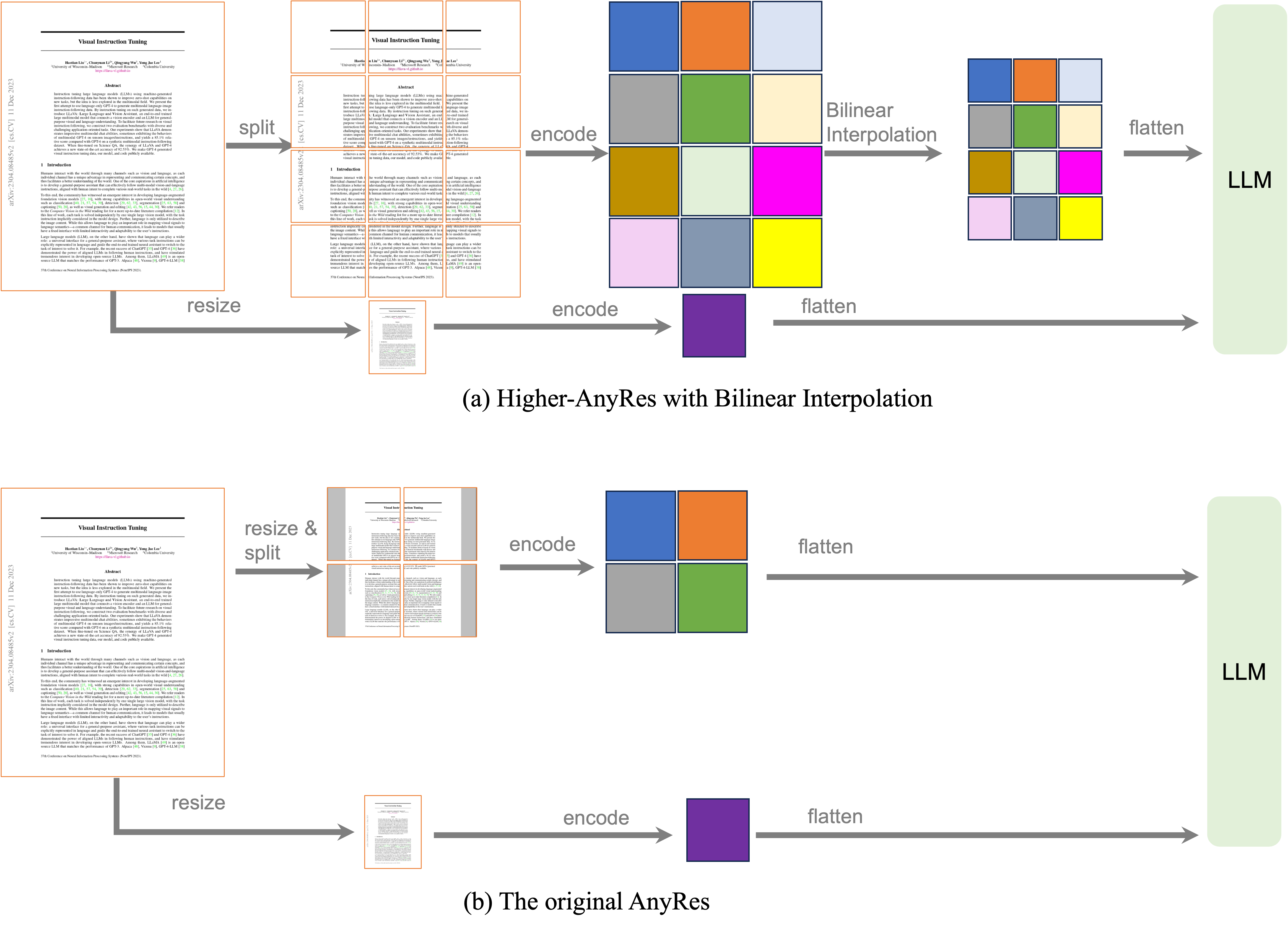
The previous AnyRes technique employs a grid configuration of \(\{2×2, 1×\{2,3,4\}, \{2,3,4\}×1\}\) to adapt to images of different resolutions while preserving data efficiency. However, this grid configuration supports a maximum of 4 grids per image, limiting its capability when more grids are required, such as with document data and long videos. As shown in Fig. 1 (a), for images with resolutions higher than the maximum supported \(768 \times 768\), the original AnyRes method resizes them to \(768 \times 768\). This resizing results in a loss of detail for high-resolution images. To address this issue, we explore grid configurations for higher resolutions, as shown in the bottom row of Fig. 1 (b), where the image is divided into more grids. Additionally, to maintain efficiency, we propose an thresholded bilinear interpolation strategy to prevent an excessive number of visual tokens from being fed into the LLM.
[Fold / Unfold to See the Details of Baseline Experiment Settings with SO400M + Qwen-1.5 0.5B]
| Configurations | ||
|---|---|---|
| Architecture |
Image Encoder: Google SO4000M (384x384) Connector: 2-Layer Relu MLP LLM: Qwen-1.5 0.5B |
|
| # Total parameters | 0.9B | |
| Visual Representations | Dynamic: 336 x {2×2,1×{2,3},{2,3}×1} | |
| Stage-1 | Training Data | 558K |
| Trainable Module | Connector | |
| Stage-2 | Training Data | 790K |
| Trainable Module | Full model | |
| Training Data (# samples) | 1348K = 558K+790K | |
| Training Schedule | Learning rate | LLM: 2e-5 / Vision: 2e-6 |
| Batch Size | 64 | |
Thresholded Bilinear Interpolation. For AnyRes with a grid configuration of width \(a\), height \(b\), and #token \(T\) per grid, the total number of visual tokens in is \(L=(a\times b + 1)\times T\). We consider a threshold \(\tau\), and reduce the #token per grid, using bilinear interpolation if needed:
$$ T_{\text{new}} = \begin{cases} \tau / ({a \times b + 1}) & \text{if } L > \tau \\ T & \text{if } L \leq \tau \end{cases}$$
Impact on Max. #Grids in Anyres and Max. #Tokens. We study the influence of resolution and #tokens on training time, and summarize the insights below.
| Max. #Grids | Max. #Tokens | Training Time | Interpolation | AI2D | ChartQA | DocVQA | InfoVQA | Image-DC | *Video-DC | **SynDOG | OK-VQA | ***POPE | ScienceQA | VizWiz-VQA | MMMU |
|---|---|---|---|---|---|---|---|---|---|---|---|---|---|---|---|
| test | test | val | val | EN | 32 frames | EN/TED Score | val | Test/F1-score | img | val | val | ||||
| 2x2 | (4+1)*729 | 6H30M | FALSE | 51.1 | 49.2 | 58.8 | 25.7 | 71.1 | 64.1 | 425.7 | 36.5 | 85.4 | 59.6 | 29.2 | 28.2 |
| 4x4 | (4+1)*729 | 7H30M | TRUE | 52.8 | 49.4 | 58.1 | 26.0 | 69.9 | 63.5 | 433.6 | 36.0 | 85.8 | 57.9 | 31.0 | 28.6 |
| 5x5 | (4+1)*729 | 7H50M | 52.4 | 49.6 | 57.6 | 26.9 | 72.9 | 63.8 | 435.6 | 36.5 | 86.1 | 58.5 | 28.7 | 28.4 | |
| 6x6 | (4+1)*729 | 8H05M | 52.7 | 50.1 | 56.7 | 27.1 | 71.0 | 64.2 | 437.2 | 35.9 | 85.9 | 58.4 | 32.2 | 28.3 | |
| 6x6 | (9+1)*729 | 11H14M | 52.7 | 55.8 | 62.7 | 26.7 | 71.7 | 64.6 | 438.9 | 42.0 | 86.1 | 58.7 | 34.7 | 29.3 | |
| 6x6 | (16+1)*729 | 13H10M | 52.7 | 56.1 | 62.2 | 27.1 | 70.2 | 65.2 | 443.5 | 42.5 | 87.4 | 58.2 | 32.8 | 27.4 |
*Video Detailed Caption Task is a new benchmark we constructed to evaluate the model's detailed captioning ability towards given images. The task is described in the Datasets Card section.
**SynDOG is a benchmark that evaluates model's OCR ability, we report the tree edit distance score on SynDOG's OCR task.
***POPE is a benchmark that evaluates model's ability on judging the existence of a given object in an image, we report the F1 score on POPE.
- We increase the maximum number of AnyRes grids from 2×2 to 6×6 to better support higher resolution, and observe that increasing #grids can enhance performance on tasks that require reading image details, such as InfoVQA and SynDOG (en). It also leads to improved performance on Video Detail Captions with 32 frames. This is because longer vision sequences are observed during training, the capability can improve video tasks with zero-shot modality transfer, based on the insights in our video blog.
- Increasing the maximum resolution causes a slighter increase in training time compared with the cost of increasing the max #tokens. Increasing max #tokens while keeping the maximum #grid 6x6 at can significantly improve OCR capability, such as ChartQA and DocVQA. We suggest prioritizing resolution over #token as a better trade-off in enriching visual representations.
Effectinveness with LLM Scaling. We further verify that the performance gains from the new visual representation persist as the LLM size scales. This is confirmed by the observation of consistent improvements across InfoVQA, ChartQA, DocVQA, VDD (32 frames), and SynDOG.
| LLM (Qwen-1.5) | Max. #Grids | Max. #Tokens | Interp. | AI2D | ChartQA | DocVQA | InfoVQA | Image-DC | Video-DC | SynDOG | OKVQA | POPE | ScienceQA | VizWiz-VQA | MMMU |
|---|---|---|---|---|---|---|---|---|---|---|---|---|---|---|---|
| test | test | val | val | EN | 32 frames | EN/TED Score | val | Test/F1-score | IMG | val | val | ||||
| 0.5B | 2x2 | (4+1)*729 | FALSE | 51.1 | 49.2 | 58.8 | 25.7 | 71.1 | 62.4 | 418.5 | 36.5 | 85.1 | 59.5 | 28.8 | 28.2 |
| 0.5B | 6x6 | (9+1)*729 | TRUE | 52.7 | 55.8 | 62.7 | 26.7 | 71.7 | 62.4 | 443.5 | 42.0 | 86.1 | 58.7 | 34.7 | 29.3 |
| 1.8B | 2x2 | (4+1)*729 | FALSE | 61.9 | 56.2 | 66.0 | 30.5 | 80.1 | 70.2 | 447.1 | 43.6 | 86.9 | 63.7 | 51.0 | 32.0 |
| 1.8B | 6x6 | (9+1)*729 | TRUE | 60.9 | 56.7 | 67.5 | 31.3 | 82.0 | 71.0 | 459.1 | 46.5 | 86.9 | 64.4 | 48.8 | 32.6 |
| 4B | 2x2 | (4+1)*729 | FALSE | 71.5 | 65.0 | 73.8 | 34.8 | 84.2 | 74.5 | 456.7 | 47.5 | 87.1 | 71.1 | 58.7 | 34.4 |
| 4B | 6x6 | (9+1)*729 | TRUE | 70.2 | 65.0 | 77.2 | 41.1 | 86.3 | 76.4 | 467.7 | 50.6 | 86.3 | 70.1 | 58.0 | 32.0 |
| 7B | 2x2 | (4+1)*729 | FALSE | 72.9 | 66.3 | 75.5 | 36.9 | 87.9 | 69.8 | 458.2 | 50.2 | 86.9 | 71.2 | 61.4 | 37.2 |
| 7B | 6x6 | (9+1)*729 | TRUE | 71.7 | 69.5 | 79.0 | 36.4 | 86.4 | 71.4 | 467.1 | 47.9 | 87.3 | 70.2 | 57.4 | 37.2 |
| 14B | 2x2 | (4+1)*729 | FALSE | 77.6 | 72.2 | 80.0 | 44.4 | 89.6 | 74.2 | 460.8 | 57.7 | 87.3 | 78.9 | 64.2 | 44.2 |
| 14B | 6x6 | (9+1)*729 | TRUE | 76.1 | 74.0 | 83.6 | 46.9 | 87.8 | 78.1 | 470.4 | 53.2 | 87.9 | 76.7 | 61.5 | 40.3 |
[Further Exploration in Resolution and Pooling (Fold / Unfold to see the Details)]
Enlarging the original images. Note that in our higher AnyRes method, we do not increase the image resolution itself. Instead, we use grid configurations that support higher resolutions. We explore how increasing image resolution affects performance and training time. As shown in the following table, increasing image resolution significantly increases training time, but does not improve performance.
| Max. # Anyres Grids | Force Resolution lifting | Min. Long Edge | Max. Tokens | Training Time | Pooling | AI2D | ChartQA | DocVQA | InfoVQA | OKVQA | POPE | ScienceQA | VizWiz-VQA |
|---|---|---|---|---|---|---|---|---|---|---|---|---|---|
| test | test | val | val | val | Test/F1-score | IMG | val | ||||||
| 4x4 | FALSE | - | (4+1)*729 | 7h30min | TRUE | 52.8 | 49.4 | 58.1 | 26.0 | 36.0 | 85.8 | 57.9 | 31.0 |
| 4x4 | TRUE | 384*4 | (4+1)*729 | 10h40min | TRUE | 52.5 | 47.9 | 58.9 | 27.0 | 34.8 | 86.5 | 58.9 | 26.0 |
| 6x6 | FALSE | - | (4+1)*729 | 8h05min | TRUE | 52.7 | 50.1 | 56.7 | 27.1 | 35.9 | 85.9 | 58.4 | 32.2 |
| 6x6 | TRUE | 384*6 | (4+1)*729 | 16h30min | TRUE | 52.1 | 48.8 | 58.5 | 26.5 | 35.0 | 86.3 | 58.7 | 26.6 |
| 6x6 | FALSE | - | (9+1)*729 | 11h14min | TRUE | 52.7 | 55.8 | 62.7 | 26.7 | 42.0 | 86.1 | 58.7 | 34.7 |
| 6x6 | TRUE | 384*6 | (9+1)*729 | 21h28min | TRUE | 52.1 | 52.3 | 62.2 | 26.6 | 40.6 | 85.5 | 57.6 | 34.1 |
Efficient strategy. For applications that require high efficiency, we explore cost-effective strategies. In the following experiment, we pool the feature map for each grid to \(t^\prime=1/4 t\). This significantly reduces training costs, although it also significantly reduces performance on high-resolution datasets such as InfoVQA, ChartQA, and DocVQA. However, performance on other datasets is either maintained or only slightly reduced. Therefore, if high efficiency is needed for low-resolution data, this setting can be considered.
| Max. #Grids | Max. #Tokens | Training Time | Pooling | Pooling After Projector | AI2D | ChartQA | DocVQA | InfoVQA | OKVQA | POPE | ScienceQA | VizWiz-VQA |
|---|---|---|---|---|---|---|---|---|---|---|---|---|
| test | test | val | val | val | Test/F1-score | IMG | val | |||||
| 2x2 | (4+1)*729 | 6h30min | FALSE | - | 51.1 | 49.2 | 58.8 | 25.7 | 36.5 | 85.4 | 59.6 | 29.2 |
| (4+1)*183 | 4h12min | TRUE | FALSE | 52.2 | 38.0 | 46.9 | 23.4 | 35.1 | 85.0 | 58.5 | 28.8 | |
| (4+1)*183 | 4h15min | TRUE | TRUE | 50.9 | 37.0 | 45.4 | 23.2 | 32.3 | 85.3 | 58.2 | 27.0 | |
| 6x6 | (4+1)*729 | 8h05min | TRUE | - | 52.7 | 50.1 | 56.7 | 27.1 | 35.9 | 85.9 | 58.4 | 32.2 |
| (4+1)*183 | 5h45min | TRUE | FALSE | 50.2 | 37.2 | 41.8 | 23.7 | 31.9 | 85.5 | 57.1 | 33.6 | |
| (4+1)*183 | 5h52min | TRUE | TRUE | 50.7 | 38.4 | 42.5 | 24.3 | 32.2 | 85.1 | 56.6 | 32.7 |
Inference. We investigated the impact of adjusting the maximum number of grids in AnyRes and visual tokens during inference, based on both performance metrics and inference time. Our findings reveal that augmenting the number of AnyRes grids during inference substantially prolongs inference time without commensurate improvements in performance. Conversely, reducing the quantity of AnyRes grids during inference diminishes performance particularly on high-resolution datasets, albeit with negligible effects on other datasets. Notably, our investigation unveiled a compelling revelation: when the maximum number of AnyRes grids for inference is set at 1x1, employing the AnyRes strategy, which utilizes (1+1)*729 visual tokens fed to the LLM, yields superior performance compared to non-AnyRes usage, where only 729 visual tokens are employed. Interestingly, despite the similarity in inference time between the two strategies, the latter exhibits superior performance. This finding underscores the importance of employing the AnyRes strategy during inference to enhance performance.
| Training | Inference | Total Inference Time | AI2D | ChartQA | DocVQA | InfoVQA | OKVQA | POPE | ScienceQA | VizWiz-VQA | MMMU | ||
|---|---|---|---|---|---|---|---|---|---|---|---|---|---|
| Max. #Grids | Max. #Tokens | Max. #Grids | Max. #Tokens | test | test | val | val | val | Test/F1-score | IMG | val | dev | |
| 2x2 | (4+1)*729 | 1x1 | 729 | ~16min | 51.2 | 29.0 | 37.3 | 19.9 | 36.6 | 80.8 | 60.3 | 31.1 | 27.2 |
| 1x1 | (1+1)*729 | ~16min | 51.2 | 33.3 | 44.9 | 20.9 | 37.5 | 82.1 | 59.3 | 31.9 | 29.7 | ||
| 2x2 | (4+1)*729 | ~20min | 51.1 | 49.2 | 58.8 | 25.7 | 36.5 | 85.4 | 59.6 | 29.2 | 28.2 | ||
| 4x4 | (4+1)*729 | ~24min | 51.7 | 45.2 | 53.4 | 26.5 | 36.5 | 85.7 | 59.0 | 29.3 | 28.4 | ||
| 4x4 | (9+1)*729 | ~27min | 51.4 | 41.1 | 51.4 | 25.4 | 36.5 | 85.7 | 59.0 | 31.4 | 28.8 | ||
| 4x4 | (16+1)*729 | 1x1 | (1+1)*729 | ~16min | 52.3 | 31.6 | 43.9 | 21.4 | 25.5 | 82.9 | 58.8 | 33.2 | 27.9 |
| 2x2 | (4+1)*729 | ~20min | 52.7 | 48.1 | 57.6 | 24.9 | 35.8 | 85.9 | 57.4 | 31.5 | 28.1 | ||
| 4x4 | (4+1)*729 | ~24min | 52.8 | 49.4 | 58.1 | 26.0 | 36.0 | 85.8 | 57.9 | 31.0 | 28.6 | ||
| 4x4 | (9+1)*729 | ~27min | 52.5 | 47.4 | 55.8 | 25.0 | 36.0 | 86.0 | 57.9 | 32.0 | 28.3 | ||
| 6x6 | (9+1)*729 | ~33min | 52.7 | 46.5 | 55.5 | 24.9 | 35.8 | 85.9 | 57.4 | 32.1 | 27.9 | ||
| 6x6 | (9+1)*729 | 1x1 | (1+1)*729 | ~16min | 53.0 | 29.8 | 44.3 | 20.1 | 40.4 | 84.5 | 58.2 | 36.3 | 30.3 |
| 2x2 | (4+1)*729 | ~20min | 52.8 | 48.3 | 59.0 | 24.6 | 42.0 | 86.2 | 58.7 | 35.1 | 30.0 | ||
| 4x4 | (4+1)*729 | ~24min | 53.2 | 48.7 | 58.1 | 25.5 | 42.0 | 86.1 | 58.5 | 35.9 | 29.7 | ||
| 6x6 | (4+1)*729 | ~30min | 52.6 | 50.1 | 55.8 | 25.1 | 42.0 | 86.2 | 58.7 | 35.8 | 29.9 | ||
| 6x6 | (9+1)*729 | ~33min | 52.7 | 55.8 | 62.7 | 26.7 | 42.0 | 86.1 | 58.7 | 34.7 | 29.3 | ||
Pooling methods: We compare adaptive average pooling and bilinear interpolation as pooling methods based on our thresholded pooling strategy. The results show that bilinear interpolation leads to better performance than adaptive average pooling does with our thresholded pooling strategy. We also compare polling Before and After projector and find that pooling After projector leads to better performance.
| Max. # Grids | Max. # Tokens | Training Time | Pooling Methods | Pooling wrt. Projector | AI2D | ChartQA | DocVQA | InfoVQA | OKVQA | POPE | ScienceQA-IMG | VizWiz |
|---|---|---|---|---|---|---|---|---|---|---|---|---|
| test | test | val | val | val | test/f1-score | img | val | |||||
| 2x2 | (4+1)*729 | 6h30min | - | - | 51.1 | 49.2 | 58.8 | 25.7 | 36.5 | 85.4 | 59.6 | 29.2 |
| 4x4 | (4+1)*729 | 7h30min | Bilinear Interpolation | After | 52.8 | 49.4 | 58.1 | 26.0 | 36.0 | 85.8 | 57.9 | 31.0 |
| Before | 48.5 | 45.4 | 50.0 | 25.4 | 30.6 | 84.5 | 56.1 | 21.6 | ||||
| AdaptiveAVGPool | After | 49.3 | 47.3 | 55.5 | 25.6 | 31.4 | 86.2 | 58.7 | 34.6 | |||
| Before | 49.2 | 43.4 | 52.7 | 25.8 | 29.8 | 84.3 | 56.2 | 22.7 | ||||
| (9+1)*729 | 48.0 | 53.2 | 57.7 | 25.5 | 37.7 | 85.8 | 56.9 | 35.2 | ||||
| (16 + 1)*729 | - | 48.7 | 54.2 | 61.2 | 24.9 | 36.9 | 86.3 | 58.9 | 36.7 | |||
| 6x6 | (9+1)*729 | 11h14min | Bilinear Interpolation | After | 52.7 | 55.8 | 62.7 | 26.7 | 42.0 | 86.1 | 58.7 | 34.7 |
| Before | 48.7 | 53.2 | 56.3 | 26.2 | 34.5 | 85.3 | 56.3 | 28.7 | ||||
| AdaptiveAVGPool | After | 48.6 | 53.0 | 59.0 | 27.4 | 37.6 | 86.0 | 58.8 | 31.2 | |||
| Before | 49.0 | 53.1 | 56.0 | 26.9 | 36.8 | 85.5 | 56.1 | 27.2 | ||||
| 6x6 | (16 + 1)*729 | 13h10min | Bilinear Interpolation | After | 52.7 | 56.1 | 62.2 | 27.1 | 42.5 | 87.4 | 58.2 | 32.8 |
| Before | 49.1 | 54.2 | 55.9 | 26.3 | 35.1 | 86.2 | 56.5 | 30.3 | ||||
| AdaptiveAVGPool | After | 48.6 | 53.0 | 59.0 | 27.4 | 37.6 | 86.0 | 58.8 | 31.2 | |||
| Before | 48.4 | 52.6 | 57.1 | 26.6 | 32.5 | 85.7 | 55.2 | 32.0 |
We then compare the two pooling methods with fixed pooling ratio \(\frac{1}{2}\). In the first row, the max. number of grids is \(4\times 4=16\) and there is no resolution lifting or pooling. In the second row, there is no resolution lifting and we directly pool the feature map to 1/2 of the original size and the performance drops significantly. Then, in the third row, we lift the resolution, letting the longer side be at least \(2\times 384=768\). The results increased compared to the second row. We then increase the max. Number of grids to \(6\times 6=36\) and lift the long side to be at least \(4\times 384=1536\). In the fourth to seventh row, we repeat the process for a larger number of grids and larger resolution. The results show that the performance increases significantly with the number of grids and the resolution.
| Max. # Grids | Increased Resolution |
Longer Side | Max. # Tokens | Pooling ratio | Pooling | Pooling wrt. Projector | Pooling Methods | AI2D | ChartQA | DocVQA | InfoVQA | OKVQA | POPE | ScienceQA | VizWiz-VQA |
|---|---|---|---|---|---|---|---|---|---|---|---|---|---|---|---|
| test | test | val | val | val | test/f1-score | img | val | ||||||||
| 4x4 | FALSE | - | (16+1)*729 | - | FALSE | - | - | 48.7 | 54.2 | 61.2 | 24.9 | 36.9 | 86.3 | 58.9 | 36.7 |
| 4x4 | FALSE | - | (4+1)*729 | 1/2 | TRUE | Before | AdaptiveAVGPool | 49.0 | 40.1 | 52.9 | 23.3 | 31.9 | 85.0 | 58.7 | 33.6 |
| 4x4 | TRUE | 2*384 | 50.0 | 40.4 | 53.4 | 24.0 | 30.4 | 85.3 | 57.8 | 38.5 | |||||
| 6x6 | TRUE | 4*384 | (9+1)*729 | 1/2 | TRUE | Before | AdaptiveAVGPool | 49.9 | 43.7 | 56.2 | 25.3 | 29.4 | 85.6 | 59.4 | 30.3 |
| After | 50.4 | 51.6 | 58.5 | 25.6 | 38.0 | 85.7 | 58.8 | 35.5 | |||||||
| Before | Bilinear Interpolation | 49.4 | 46.2 | 56.4 | 26.6 | 34.1 | 86.1 | 59.8 | 29.1 | ||||||
| After | 50.6 | 42.7 | 55.7 | 27.7 | 30.4 | 85.9 | 59.4 | 27.9 |
Section 3 - Insights on Training Strategies
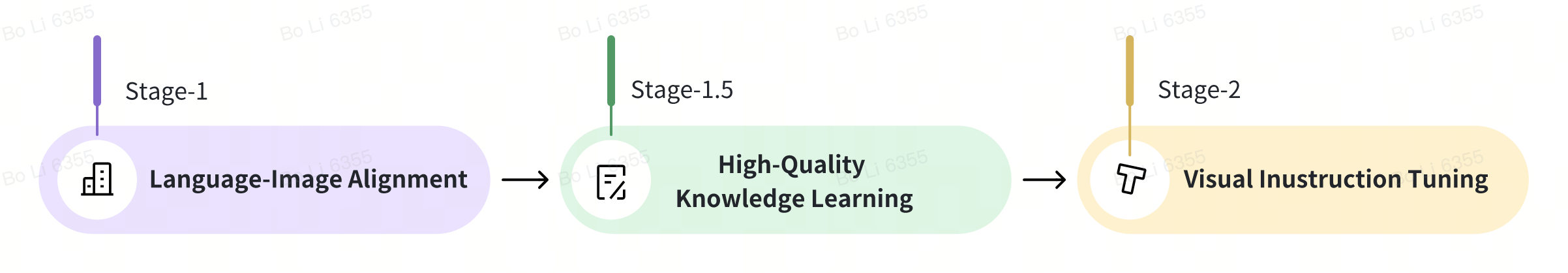
To enable LLM for multimodal capabilities, we identify three critical functionalities, and systematically divide them into three distinct learning stages for the purpose of ablation studies. As with most existing research, prior LLaVA models mainly explore Stage-2 for new scenarios and improved performance. However, the first two functionalities are less frequently investigated and therefore constitute the primary focus of this section.
- Stage-1: Language-Image Alignment.
- Stage-1.5: High-Quality Knowledge Learning.
- Stage-2: Visual Instruction Tuning.
[Fold / Unfold to See the Details of Baseline Experiment Settings with CLIP-L-336 + Vicuna-1.5 7B]
| Configurations | ||
|---|---|---|
| Architecture |
Image Encoder: OpenAI CLIP-Large (336x3336) Connector: 2-Layer Relu MLP LLM: Vicuna-1.5 7B |
|
| # Total parameters | 7.06B | |
| Visual Representations | Dynamic: 336 x {2×2,1×{2,3},{2,3}×1} | |
| Stage-1 | Training Data | 558K |
| Trainable Module | Connector | |
| Stage-1.5 | Training Data | - |
| Trainable Module | Full model | |
| Stage-2 | Training Data | 790K |
| Trainable Module | Full model | |
| Training Data (# samples) | 1348K = 558K+790K | |
| Training Schedule | Learning rate | LLM: 2e-5 / Vision: 2e-6 |
| Batch Size | 128 | |
Section 3.1 - Language-Image Alignment
We considered two groups of data to align the image features into the text embedding space:
- Public Data: BLIP558K, CC3M, and CC12M.
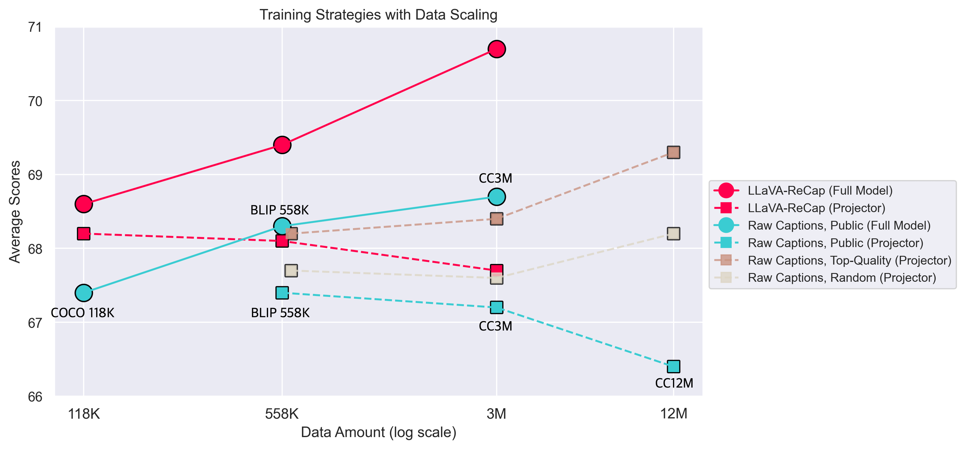
- Web Data: to avoid the limitations imposed by the quantity of existing public data, we consider multimodal image-text data from the internet at similar scales. We applied quality control measures to filter this data to match public data at similar scales of 0.6M, 3M and 12M. The well-trained projector is used directly to run full model tuning with visual instructions, and the results are reported below. With tuning the projector only, the data scaling is less effective with public raw data, while more effective with top-quality data mixture, followed by the randomly selected data mixture from the same web dataset.
| Stage-1 Data | Quality Measure | Avg. | AI2D* | ChartQA* | DocVQA | MathVista | MME | LLaVA-W | ScienceQA | Image-DC |
|---|---|---|---|---|---|---|---|---|---|---|
| - | test | test | val | testmini | - | - | IMG | EN | ||
| 558K | N/A | 67.4 | 67.4 | 65.2 | 74.5 | 35.4 | 65.54 | 72.6 | 71.0 | 87.6 |
| CC3M | N/A | 67.2 | 66.0 | 62.4 | 73.7 | 35.4 | 66.60 | 79.9 | 69.5 | 84.3 |
| CC12M | N/A | 66.4 | 66.8 | 58.9 | 72.5 | 34.7 | 64.14 | 79.6 | 69.7 | 85.1 |
| Web Dataset* | ||||||||||
| Web 0.6M | Top Quality | 68.2 | 67.8 | 64.8 | 74.2 | 35.2 | 66.61 | 80.1 | 71.4 | 85.4 |
| Random | 67.7 | 68.0 | 64.4 | 73.7 | 34.4 | 65.83 | 80.6 | 70.8 | 83.7 | |
| Web 3M | Top Quality | 68.4 | 67.8 | 62.9 | 73.8 | 34.1 | 67.05 | 86.4 | 70.3 | 84.5 |
| Random | 67.6 | 68.2 | 62.8 | 73.2 | 33.4 | 66.00 | 83.0 | 70.1 | 84.3 | |
| Web 12M | Top Quality | 69.3 | 68.6 | 64.5 | 74.9 | 35.8 | 69.34 | 85.2 | 71.0 | 85.1 |
| Random | 68.2 | 68.2 | 62.4 | 73.4 | 34.1 | 66.87 | 85.6 | 70.9 | 83.8 | |
Section 3.2 - High-Quality Knowledge Learning
In the realm of multimodal training from LLM, the axiom "quality over quantity" holds especially true. This principle is paramount due to the extensive knowledge stored within pre-trained LLM and ViT. While it is essential to accumulate balanced, diverse, and high-quality instruction data at the end of the LMM's training lifecycle, an often-overlooked aspect is the continuous exposure of the model to new, high-quality data for further knowledge acquisition, when it is available. We term Stage-1.5, focuses on high-quality knowledge learning. The training configuration mirrors the settings used in Stage-2, ensuring consistency and allowing the model to integrate new information seamlessly. This approach acknowledges that the pre-trained LLMs and ViTs already possess a substantial knowledge base, and the goal is to refine and enhance this knowledge with carefully curated data. By prioritizing the quality of data, we can maximize compute efficiency.
To illustrate high-quality knowledge, we consider data from three major categories:
- Re-Captioned Detailed Description Data: LLaVA-NeXT-34B is known for its strong detailed caption ability among open-source LMMs. We used the model to generate new captions for the images from the following datasets: COCO118K, BLIP558K, and CC3M.
- Document / OCR Data: We utilized the Text Reading subset from the UReader dataset, totaling 100K, which is easily accessible through PDF rendering. We used this text reading data along with the SynDOG EN/CN 1M datasets.
- ShareGPT4V Chinese Detailed Caption: We used the original ShareGPT4V[3] images and utilized GPT-4V provided by the Azure API to generate detailed Chinese caption data, aiming to improve the model's capability in Chinese.
Here are more detailed ablations, and the following tables may present the following conclusions:
-
Enhanced Performance with Recaptioned Data: Models trained with recaptioned data
(ReCap) datasets, show a trend of enhanced performance in tasks requiring detailed image descriptions
and document understanding.
- The regenerated captions, ranging from 118K to 3M, demonstrate better scaling behaviors than the original captions, consistently improve model performance across various metrics.
- With recap data, full-model training is more effective than projector tuning, because larger model capacity is needed to digest high-quality knowledge. This approach results in notable improvements in metrics like AI2D, DocVQA, ChartQA, InfoVQA, and ScienceQA.
-
Enhancement through New Domain Knowledge: The introduction of new domain knowledge is
essential.
- Document/OCR data, particularly UReader 100K and SynDOG EN/CN 1M, provide substantial benefits in understanding structured text data.
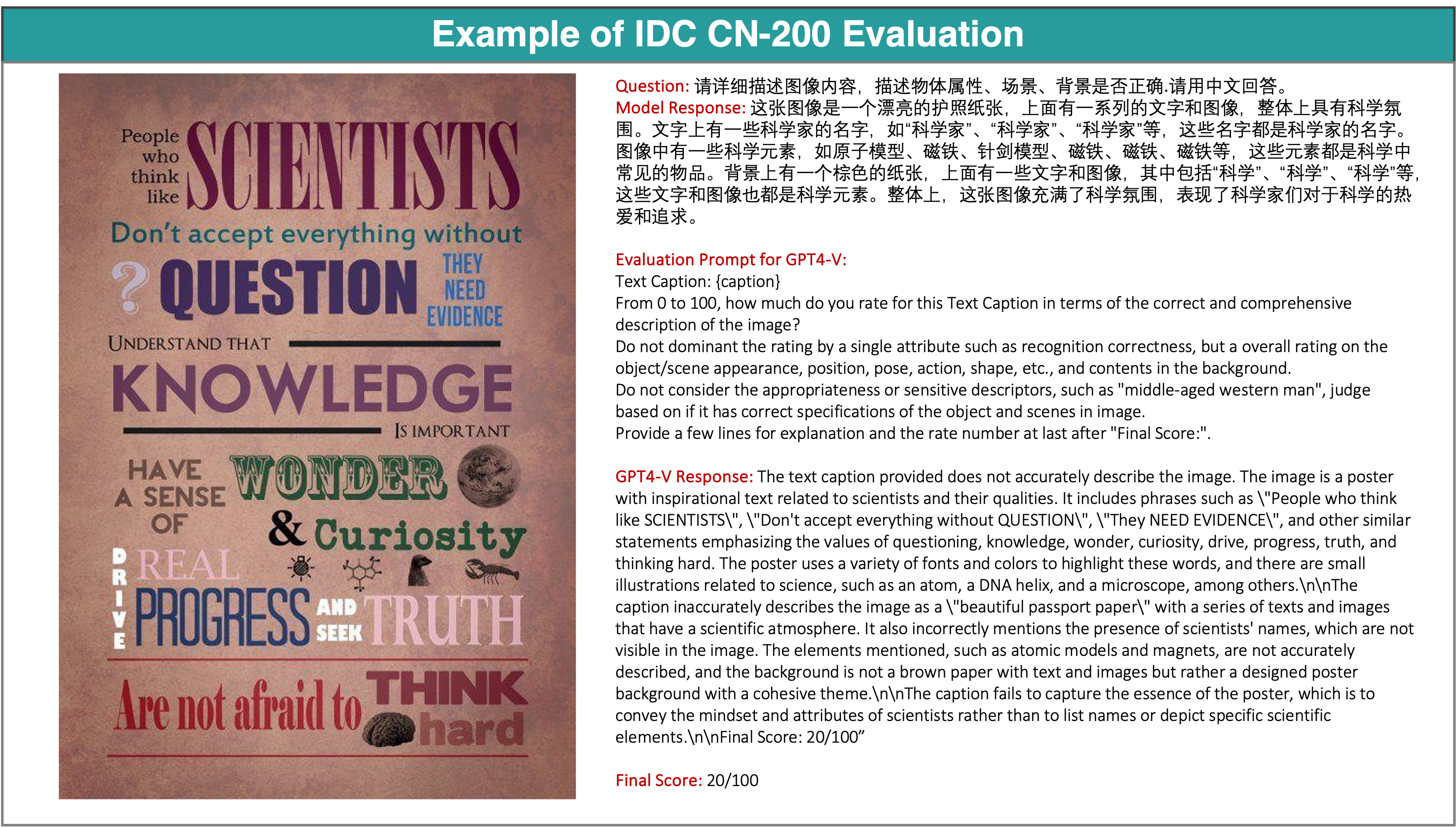
- ShareGPT4V Chinese Caption data, enhances the model's ability to understand and process multilingual data. This improvement is evident in the increased scores across several metrics, especially in the Chinese version of Image-DC and CMMU, demonstrating the model's enhanced multilingual capabilities.
- Balanced Improvement with Mixed Data Approach: Combining high-quality recaptioned data, document data, and text data (e.g., Recap-118K, UReader 100K, and Evol-Instruct) leads to a well-rounded model capable of performing well across diverse tasks. Despite the total amount being under 500K, this efficient mixed data approach results in balanced improvements across most metrics. This suggests that a comprehensive and diverse knowledge base is crucial for the effectiveness of multimodal models.
| Training Data | Avg. | AI2D | ChartQA | DocVQA | InfoVQA | MathVista | MME | LLaVA-W | ScienceQA | Image-DC | ||
|---|---|---|---|---|---|---|---|---|---|---|---|---|
| Stage-1 | Stage 1.5 | Stage 2 | - | test | test | val | val | testmini | - | - | IMG | EN |
| 558K | - | 790K | 67.4 | 67.4 | 65.2 | 74.5 | 34.5 | 35.4 | 65.5 | 72.6 | 70.8 | 87.5 |
| High-Quality Knowledge: Detailed Re-Captioning | ||||||||||||
| 118K (ReCap) | - | 790K | 68.2 | 66.9 | 65.2 | 75.3 | 36.7 | 35.6 | 65.1 | 79.8 | 69.7 | 88.2 |
| 558K (ReCap) | - | 68.1 | 66.7 | 66.0 | 74.6 | 36.2 | 34.4 | 64.9 | 79.4 | 72.3 | 86.3 | |
| 3M (ReCap) | - | 67.7 | 66.1 | 66.2 | 74.3 | 35.5 | 35.1 | 64.4 | 79.9 | 71.2 | 84.3 | |
| 558K | 118K (ReCap) | 68.6 | 66.9 | 66.6 | 75.5 | 36.6 | 36.1 | 65.7 | 79.7 | 71.0 | 87.6 | |
| 558K (ReCap) | 69.4 | 70.1 | 67.8 | 76.9 | 39.4 | 36.2 | 65.1 | 79.4 | 71.5 | 88.2 | ||
| 3M (Recap) | 70.7 | 72.7 | 68.3 | 77.7 | 38.1 | 38.6 | 65.7 | 80.1 | 72.0 | 90.4 | ||
| COCO118K | 67.4 | 66.1 | 65.7 | 73.7 | 35.1 | 35.5 | 65.8 | 75.9 | 70.1 | 86.2 | ||
| BLIP558K | 68.3 | 67.3 | 66.1 | 75.4 | 36.8 | 35.8 | 66.6 | 77.6 | 70.9 | 86.6 | ||
| CC3M | 68.7 | 67.5 | 66.3 | 77.0 | 38.1 | 34.9 | 66.8 | 79.6 | 71.0 | 86.5 | ||
| High-Quality Knowledge: New Domain Knowledge | ||||||||||||
| 558K | UReader 100K | 790K | 67.2 | 66.2 | 67.2 | 77.6 | 36.9 | 34.2 | 63.9 | 70.7 | 71.9 | 86.1 |
| ShareGPT4V Chinese Caption 100K | 68.7 | 68.7 | 67.1 | 75.1 | 36.9 | 36.3 | 64.4 | 78.1 | 72.2 | 87.4 | ||
| SynDOG 1M | 66.3 | 66.4 | 62.0 | 72.9 | 36.7 | 31.6 | 65.8 | 76.9 | 72.5 | 82.3 | ||
| Mixed Data | ||||||||||||
| 558K | 118K (ReCap) + UReader |
790K | 68.9 | 66.9 | 68.1 | 79.2 | 37.8 | 36.0 | 64.2 | 77.4 | 71.0 | 88.5 |
| 118K (ReCap) + UReader + Evol-143K |
69.4 | 66.2 | 67.7 | 78.5 | 38.1 | 36.2 | 66.1 | 81.4 | 71.3 | 88.1 | ||
The table above presents the results of Chinese-related tasks, including detailed captions, CMMMU, and OCRBench (with some subsets related to Chinese evaluation).
| Training Data | Image-DC |
OCRBench | CMMU | ||
|---|---|---|---|---|---|
| Stage-1 | Stage-1.5 | Stage-2 | CN-200 | test-all | val |
| BLIP558K | - | 790K | 65.6 | 54.8 | 24.0 |
| SynDOG 1M | 55.3 | 42.6 | 21.3 | ||
| UReader 100K | 49.4 | 58.0 | 22.8 | ||
| ShareGPT4V CN-Caption 100K | 80.4 | 56.0 | 25.6 | ||
Dataset Card
In this section, we will provide detailed information of our recaptioned data and the evaluation process for the two newly added tasks.
LLaVA Recaptioned Data
We re-captioned the original data with the prompts of "Please generate detailed descriptions of the given image.". Here's the detailed information of our re-captioned data.
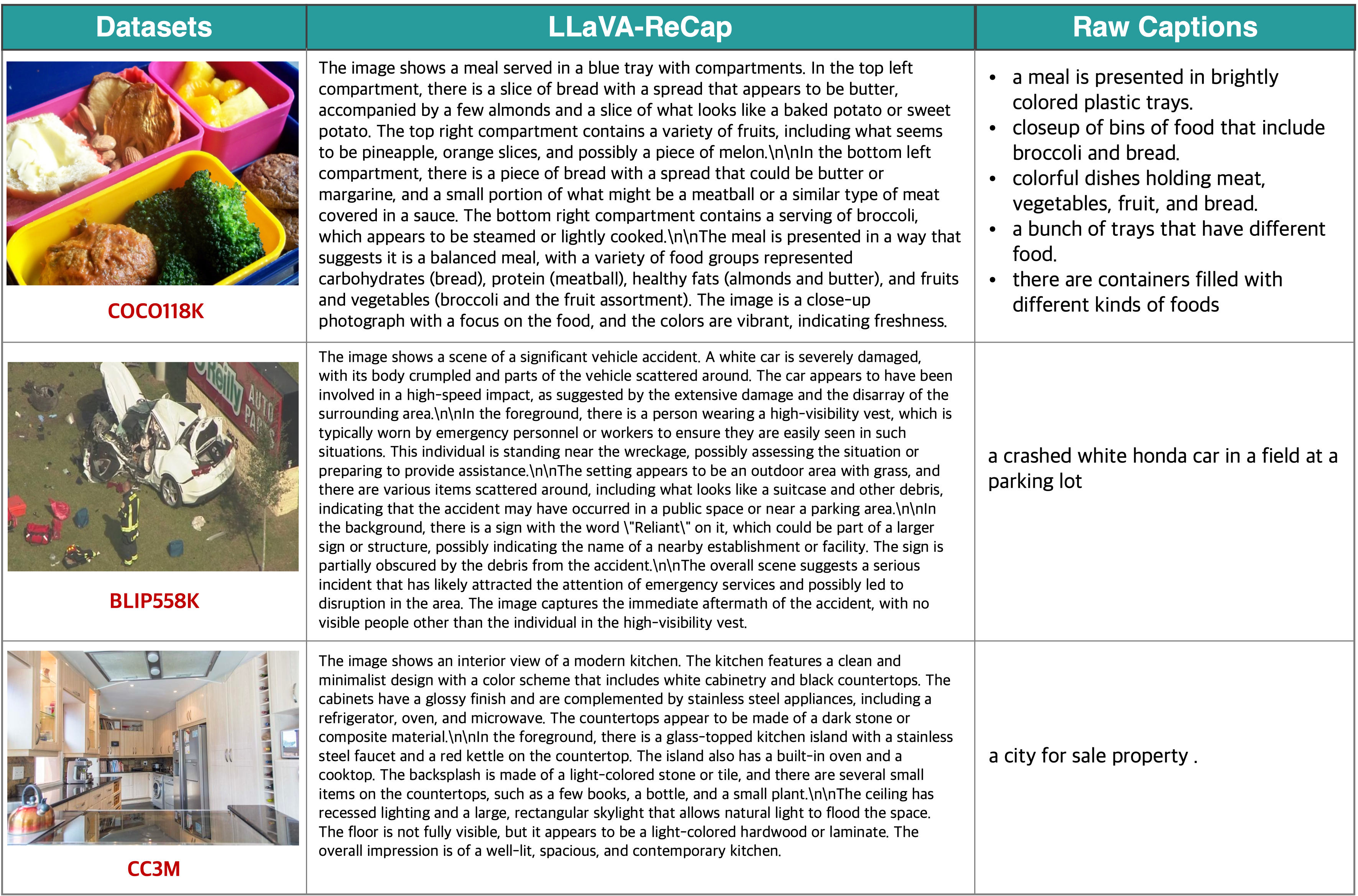
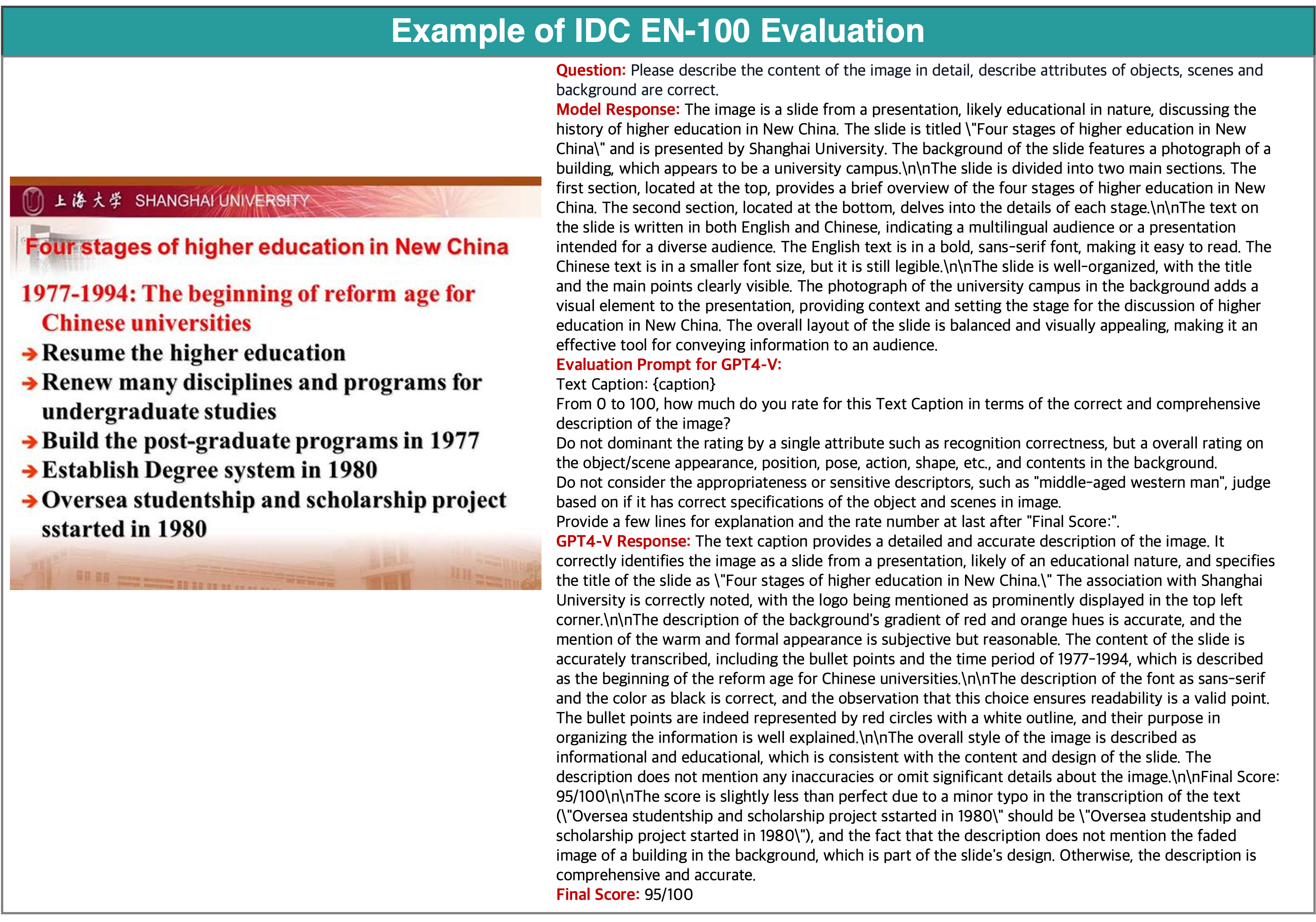
Image Detailed Caption Task
In this task, the images are from self-collected, natural and daily-life sources. And we divide our evaluations into two subsets (1) English with 100 instances. (2) Chinese with 200 instances.
Here are a few examples of this task.
[Please Fold / Unfold to Check More Examples]
While we are uncertain if this evaluation data will be publicly released, we demonstrate some examples and ensure that it is out-of-domain from all our training data and will be used solely as an internal development metric. Please do not refer to this as formal metric for comparison with other models.
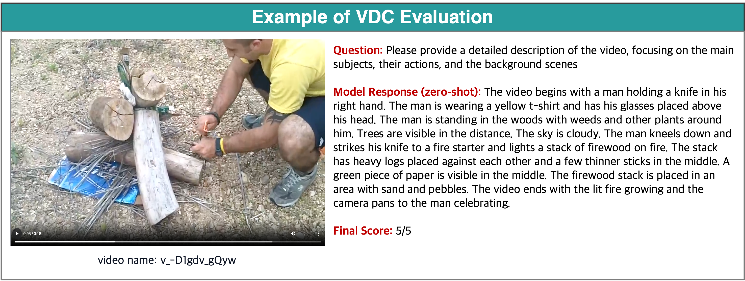
Video Detailed Caption Task
This dataset comprises 499 videos sourced from ActivityNet[4], with the evaluation process inspired by VideoChatGPT[5]. For each video, we prompt the model with: Please provide a detailed description of the video, focusing on the main subjects, their actions, and the background scenes. Ground-truth answers are extracted from the human-generated detailed descriptions of the videos. The model's responses are evaluated using a custom-designed prompt, which rates the model responses using gpt-3.5-turbo-0613.
Here are a few examples of this task.
More examples could be visited at VideoDetailedCaptions. Their evaluation process could be visited at lmms-eval (we will release and support evaluations with video datasets soon).
Reference
- Hoffmann, Jordan, et al. "Training compute-optimal large language models." arXiv preprint arXiv:2203.15556 (2022).
- Rae, Jack W., et al. "Scaling language models: Methods, analysis & insights from training gopher." arXiv preprint arXiv:2112.11446 (2021).
- Chen, Lin, et al. "Sharegpt4v: Improving large multi-modal models with better captions." arXiv preprint arXiv:2311.12793 (2023).
- Caba Heilbron, Fabian, et al. "Activitynet: A large-scale video benchmark for human activity understanding." Proceedings of the ieee conference on computer vision and pattern recognition. 2015.
- Maaz, Muhammad, et al. "Video-chatgpt: Towards detailed video understanding via large vision and language models." arXiv preprint arXiv:2306.05424 (2023).
Team
-
Bo Li*: Nanyang Technological University
 ( Work collaborated with ByteDance)
-
Hao Zhang*: Hong Kong University of Science and
Technology
 (Work collaborated with ByteDance)
-
Kaichen Zhang:
Nanyang Technological University (Work collaborated with ByteDance)
-
Dong Guo: ByteDance

-
Yuanhan Zhang: Nanyang Technological University
( Work collaborated with ByteDance)
-
Renrui Zhang: The Chinese University of Hong Kong
 (Work collaborated with ByteDance)
-
Feng Li: Hong Kong University of Science and Technology
( Work collaborated with ByteDance)
-
Ziwei Liu: Nanyang Technological University
-
Chunyuan Li: Bytedance
Related Blogs
- LLaVA-NeXT: Stronger LLMs Supercharge Multimodal Capabilities in the Wild
- LLaVA-NeXT: A Strong Zero-shot Video Understanding Model
- LLaVA-NeXT: Improved reasoning, OCR, and world knowledge
- Accelerating the Development of Large Multimodal Models with LMMs-Eval
Citation
@misc{li2024llavanext-ablations,
    title={LLaVA-NeXT: What Else Influences Visual Instruction Tuning Beyond Data?},
    url={https://llava-vl.github.io/blog/2024-05-25-llava-next-ablations/},
    author={Li, Bo and Zhang, Hao and Zhang, Kaichen and Guo, Dong and Zhang, Yuanhan and Zhang, Renrui and Li, Feng and Liu, Ziwei and Li, Chunyuan},
    month={May},
    year={2024}
}

@misc{li2024llavanext-strong,
    title={LLaVA-NeXT: Stronger LLMs Supercharge Multimodal Capabilities in the Wild},
    url={https://llava-vl.github.io/blog/2024-05-10-llava-next-stronger-llms/},
    author={Li, Bo and Zhang, Kaichen and Zhang, Hao and Guo, Dong and Zhang, Renrui and Li, Feng and Zhang, Yuanhan and Liu, Ziwei and Li, Chunyuan},
    month={May},
    year={2024}
}

@misc{zhang2024llavanextvideo,
    title={LLaVA-NeXT: A Strong Zero-shot Video Understanding Model},
    url={https://llava-vl.github.io/blog/2024-04-30-llava-next-video/},
    author={Zhang, Yuanhan and Li, Bo and Liu, haotian and Lee, Yong jae and Gui, Liangke and Fu, Di and Feng, Jiashi and Liu, Ziwei and Li, Chunyuan},
    month={April},
    year={2024}
}

@misc{liu2024llavanext,
    title={LLaVA-NeXT: Improved reasoning, OCR, and world knowledge},
    url={https://llava-vl.github.io/blog/2024-01-30-llava-next/},
    author={Liu, Haotian and Li, Chunyuan and Li, Yuheng and Li, Bo and Zhang, Yuanhan and Shen, Sheng and Lee, Yong Jae},
    month={January},
    year={2024}
}

@misc{liu2023improvedllava,
      title={Improved Baselines with Visual Instruction Tuning},
      author={Liu, Haotian and Li, Chunyuan and Li, Yuheng and Lee, Yong Jae},
      publisher={arXiv:2310.03744},
      year={2023},
}

@misc{liu2023llava,
      title={Visual Instruction Tuning},
      author={Liu, Haotian and Li, Chunyuan and Wu, Qingyang and Lee, Yong Jae},
      publisher={NeurIPS},
      year={2023},
}